Fine-tuning LSTM-based Language Model
Now that we’ve covered some advanced topics using advanced models, let’s return to the basics and show how these techniques can help us even when addressing the comparatively simple problem of classification. In particular, we’ll look at the classic problem of sentiment analysis: taking an input consisting of a string of text and classifying its sentiment as positive or negative.
In this notebook, we are going to use GluonNLP to build a sentiment analysis model whose weights are initialized based on a pre-trained language model. Using pre-trained language model weights is a common approach for semi-supervised learning in NLP. In order to do a good job with large language modeling on a large corpus of text, our model must learn representations that contain information about the structure of natural language. Intuitively, by starting with these good features, versus simply random features, we’re able to converge faster towards a superior model for our downstream task.
With GluonNLP, we can quickly prototype the model and it’s easy to customize. The building process consists of just three simple steps. For this demonstration we’ll focus on movie reviews from the Large Movie Review Dataset, also known as the IMDB dataset. Given a movie, our model will output prediction of its sentiment, which can be positive or negative.
Setup
Firstly, we must load the required modules. Please remember to download the archive from the top of this tutorial if you’d like to follow along. We set the random seed so the outcome can be relatively consistent.
[1]:
import warnings
warnings.filterwarnings('ignore')

import random
import time
import multiprocessing as mp
import numpy as np

import mxnet as mx
from mxnet import nd, gluon, autograd

import gluonnlp as nlp
nlp.utils.check_version('0.7.0')

random.seed(123)
np.random.seed(123)
mx.random.seed(123)
Sentiment analysis model with pre-trained language model encoder
So that we can easily transplant the pre-trained weights, we’ll base our model architecture on the pre-trained language model (LM). Following the LSTM layer, we have one representation vector for each word in the sentence. Because we plan to make a single prediction (as opposed to one per word), we’ll first pool our predictions across time steps before feeding them through a dense last layer to produce our final prediction (a single sigmoid output node).
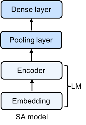
Specifically, our model represents input words by their embeddings. Following the embedding layer, our model consists of a two-layer LSTM, followed by an average pooling layer, followed by a sigmoid output layer (all illustrated in the figure above).
Thus, given an input sequence, the memory cells in the LSTM layer will produce a representation sequence. This representation sequence is then averaged over all time steps resulting in a fixed-length sentence representation \(h\). Finally, we apply a sigmoid output layer on top of \(h\). We’re using the sigmoid activation function because we’re trying to predict if this text has positive or negative sentiment. A sigmoid activation function squashes the output values to the range [0,1], allowing us to interpret this output as a probability, making our lives relatively simpler.
Below we define our MeanPoolingLayer and basic sentiment analysis network’s (SentimentNet) structure.
[2]:
class MeanPoolingLayer(gluon.HybridBlock):
    """A block for mean pooling of encoder features"""
    def __init__(self, prefix=None, params=None):
        super(MeanPoolingLayer, self).__init__(prefix=prefix, params=params)

    def hybrid_forward(self, F, data, valid_length): # pylint: disable=arguments-differ
        """Forward logic"""
        # Data will have shape (T, N, C)
        masked_encoded = F.SequenceMask(data,
                                        sequence_length=valid_length,
                                        use_sequence_length=True)
        agg_state = F.broadcast_div(F.sum(masked_encoded, axis=0),
                                    F.expand_dims(valid_length, axis=1))
        return agg_state


class SentimentNet(gluon.HybridBlock):
    """Network for sentiment analysis."""
    def __init__(self, dropout, prefix=None, params=None):
        super(SentimentNet, self).__init__(prefix=prefix, params=params)
        with self.name_scope():
            self.embedding = None # will set with lm embedding later
            self.encoder = None # will set with lm encoder later
            self.agg_layer = MeanPoolingLayer()
            self.output = gluon.nn.HybridSequential()
            with self.output.name_scope():
                self.output.add(gluon.nn.Dropout(dropout))
                self.output.add(gluon.nn.Dense(1, flatten=False))

    def hybrid_forward(self, F, data, valid_length): # pylint: disable=arguments-differ
        encoded = self.encoder(self.embedding(data))  # Shape(T, N, C)
        agg_state = self.agg_layer(encoded, valid_length)
        out = self.output(agg_state)
        return out
Defining the hyperparameters and initializing the model
Hyperparameters
Our model is based on a standard LSTM model. We use a hidden layer size of 200. We use bucketing for speeding up the processing of variable-length sequences. We don’t configure dropout for this model as it could be deleterious to the results.
[3]:
dropout = 0
language_model_name = 'standard_lstm_lm_200'
pretrained = True
learning_rate, batch_size = 0.005, 32
bucket_num, bucket_ratio = 10, 0.2
epochs = 1
grad_clip = None
log_interval = 100
If your environment supports GPUs, keep the context value the same. If it doesn’t, swap the mx.gpu(0) to mx.cpu().
[4]:
context = mx.gpu(0)
Loading the pre-trained model
The loading of the pre-trained model, like in previous tutorials, is as simple as one line.
[5]:
lm_model, vocab = nlp.model.get_model(name=language_model_name,
                                      dataset_name='wikitext-2',
                                      pretrained=pretrained,
                                      ctx=context,
                                      dropout=dropout)
Vocab file is not found. Downloading.
Downloading /root/.mxnet/models/6174723823812585603/6174723823812585603_wikitext-2-be36dc52.zip from https://apache-mxnet.s3-accelerate.dualstack.amazonaws.com/gluon/dataset/vocab/wikitext-2-be36dc52.zip...
Downloading /root/.mxnet/models/standard_lstm_lm_200_wikitext-2-b233c700.zip7148d016-223c-42d8-87fd-d194312b9e34 from https://apache-mxnet.s3-accelerate.dualstack.amazonaws.com/gluon/models/standard_lstm_lm_200_wikitext-2-b233c700.zip...
Creating the sentiment analysis model from the loaded pre-trained model
In the code below, we already have acquireq a pre-trained model on the Wikitext-2 dataset using nlp.model.get_model. We then construct a SentimentNet object, which takes as input the embedding layer and encoder of the pre-trained model.
As we employ the pre-trained embedding layer and encoder, we only need to initialize the output layer using net.out_layer.initialize(mx.init.Xavier(), ctx=context).
[6]:
net = SentimentNet(dropout=dropout)
net.embedding = lm_model.embedding
net.encoder = lm_model.encoder
net.hybridize()
net.output.initialize(mx.init.Xavier(), ctx=context)
print(net)
SentimentNet(
  (embedding): HybridSequential(
    (0): Embedding(33278 -> 200, float32)
  )
  (encoder): LSTM(200 -> 200, TNC, num_layers=2)
  (agg_layer): MeanPoolingLayer(

  )
  (output): HybridSequential(
    (0): Dropout(p = 0, axes=())
    (1): Dense(None -> 1, linear)
  )
)
The data pipeline
In this section, we describe in detail the data pipeline, from initialization to modifying it for use in our model.
Loading the sentiment analysis dataset (IMDB reviews)
In the labeled train/test sets, out of a max score of 10, a negative review has a score of no more than 4, and a positive review has a score of no less than 7. Thus reviews with more neutral ratings are not included in the train/test sets. We labeled a negative review whose score <= 4 as 0, and a positive review whose score >= 7 as 1. As the neural ratings are not included in the datasets, we can use 5 as our threshold.
[7]:
# The tokenizer takes as input a string and outputs a list of tokens.
tokenizer = nlp.data.SpacyTokenizer('en')

# `length_clip` takes as input a list and outputs a list with maximum length 500.
length_clip = nlp.data.ClipSequence(500)

# Helper function to preprocess a single data point
def preprocess(x):
    data, label = x
    label = int(label > 5)
    # A token index or a list of token indices is
    # returned according to the vocabulary.
    data = vocab[length_clip(tokenizer(data))]
    return data, label

# Helper function for getting the length
def get_length(x):
    return float(len(x[0]))

# Loading the dataset
train_dataset, test_dataset = [nlp.data.IMDB(root='data/imdb', segment=segment)
                               for segment in ('train', 'test')]
print('Tokenize using spaCy...')
Downloading data/imdb/train.json from https://apache-mxnet.s3-accelerate.dualstack.amazonaws.com/gluon/dataset/imdb/train.json...
Downloading data/imdb/test.json from https://apache-mxnet.s3-accelerate.dualstack.amazonaws.com/gluon/dataset/imdb/test.json...
Tokenize using spaCy...
Here we use the helper functions defined above to make pre-processing the dataset relatively stress-free and concise. As in a previous tutorial, mp.Pool() is leveraged to divide the work of preprocessing to multiple cores/machines.
[8]:
def preprocess_dataset(dataset):
    start = time.time()
    with mp.Pool() as pool:
        # Each sample is processed in an asynchronous manner.
        dataset = gluon.data.SimpleDataset(pool.map(preprocess, dataset))
        lengths = gluon.data.SimpleDataset(pool.map(get_length, dataset))
    end = time.time()
    print('Done! Tokenizing Time={:.2f}s, #Sentences={}'.format(end - start, len(dataset)))
    return dataset, lengths

# Doing the actual pre-processing of the dataset
train_dataset, train_data_lengths = preprocess_dataset(train_dataset)
test_dataset, test_data_lengths = preprocess_dataset(test_dataset)
Done! Tokenizing Time=8.72s, #Sentences=25000
Done! Tokenizing Time=8.53s, #Sentences=25000
In the following code, we use FixedBucketSampler, which assigns each data sample to a fixed bucket based on its length. The bucket keys are either given or generated from the input sequence lengths and the number of buckets.
[9]:
# Construct the DataLoader

def get_dataloader():

    # Pad data, stack label and lengths
    batchify_fn = nlp.data.batchify.Tuple(
        nlp.data.batchify.Pad(axis=0, pad_val=0, ret_length=True),
        nlp.data.batchify.Stack(dtype='float32'))
    batch_sampler = nlp.data.sampler.FixedBucketSampler(
        train_data_lengths,
        batch_size=batch_size,
        num_buckets=bucket_num,
        ratio=bucket_ratio,
        shuffle=True)
    print(batch_sampler.stats())

    # Construct a DataLoader object for both the training and test data
    train_dataloader = gluon.data.DataLoader(
        dataset=train_dataset,
        batch_sampler=batch_sampler,
        batchify_fn=batchify_fn)
    test_dataloader = gluon.data.DataLoader(
        dataset=test_dataset,
        batch_size=batch_size,
        shuffle=False,
        batchify_fn=batchify_fn)
    return train_dataloader, test_dataloader

# Use the pre-defined function to make the retrieval of the DataLoader objects simple
train_dataloader, test_dataloader = get_dataloader()
FixedBucketSampler:
  sample_num=25000, batch_num=778
  key=[59, 108, 157, 206, 255, 304, 353, 402, 451, 500]
  cnt=[591, 1999, 5087, 5110, 3036, 2083, 1476, 1164, 874, 3580]
  batch_size=[54, 32, 32, 32, 32, 32, 32, 32, 32, 32]
Training the model
Now that all the data has been pre-processed and the model architecture has been loosely defined, we can define the helper functions for evaluation and training of the model.
Evaluation using loss and accuracy
Here, we define a function evaluate(net, dataloader, context) to determine the loss and accuracy of our model in a concise way. The code is very similar to evaluation of other models in the previous tutorials. For more information and explanation of this code, please refer to the previous tutorial on LSTM-based Language Models.
[10]:
def evaluate(net, dataloader, context):
    loss = gluon.loss.SigmoidBCELoss()
    total_L = 0.0
    total_sample_num = 0
    total_correct_num = 0
    start_log_interval_time = time.time()

    print('Begin Testing...')
    for i, ((data, valid_length), label) in enumerate(dataloader):
        data = mx.nd.transpose(data.as_in_context(context))
        valid_length = valid_length.as_in_context(context).astype(np.float32)
        label = label.as_in_context(context)
        output = net(data, valid_length)

        L = loss(output, label)
        pred = (output > 0.5).reshape(-1)
        total_L += L.sum().asscalar()
        total_sample_num += label.shape[0]
        total_correct_num += (pred == label).sum().asscalar()

        if (i + 1) % log_interval == 0:
            print('[Batch {}/{}] elapsed {:.2f} s'.format(
                i + 1, len(dataloader),
                time.time() - start_log_interval_time))
            start_log_interval_time = time.time()

    avg_L = total_L / float(total_sample_num)
    acc = total_correct_num / float(total_sample_num)

    return avg_L, acc
In the following code, we use FixedBucketSampler, which assigns each data sample to a fixed bucket based on its length. The bucket keys are either given or generated from the input sequence lengths and number of the buckets.
[11]:
def train(net, context, epochs):
    trainer = gluon.Trainer(net.collect_params(), 'ftml',
                            {'learning_rate': learning_rate})
    loss = gluon.loss.SigmoidBCELoss()

    parameters = net.collect_params().values()

    # Training/Testing
    for epoch in range(epochs):
        # Epoch training stats
        start_epoch_time = time.time()
        epoch_L = 0.0
        epoch_sent_num = 0
        epoch_wc = 0
        # Log interval training stats
        start_log_interval_time = time.time()
        log_interval_wc = 0
        log_interval_sent_num = 0
        log_interval_L = 0.0

        for i, ((data, length), label) in enumerate(train_dataloader):
            L = 0
            wc = length.sum().asscalar()
            log_interval_wc += wc
            epoch_wc += wc
            log_interval_sent_num += data.shape[1]
            epoch_sent_num += data.shape[1]
            with autograd.record():
                output = net(data.as_in_context(context).T,
                             length.as_in_context(context)
                                   .astype(np.float32))
                L = L + loss(output, label.as_in_context(context)).mean()
            L.backward()
            # Clip gradient
            if grad_clip:
                gluon.utils.clip_global_norm(
                    [p.grad(context) for p in parameters],
                    grad_clip)
            # Update parameter
            trainer.step(1)
            log_interval_L += L.asscalar()
            epoch_L += L.asscalar()
            if (i + 1) % log_interval == 0:
                print(
                    '[Epoch {} Batch {}/{}] elapsed {:.2f} s, '
                    'avg loss {:.6f}, throughput {:.2f}K wps'.format(
                        epoch, i + 1, len(train_dataloader),
                        time.time() - start_log_interval_time,
                        log_interval_L / log_interval_sent_num, log_interval_wc
                        / 1000 / (time.time() - start_log_interval_time)))
                # Clear log interval training stats
                start_log_interval_time = time.time()
                log_interval_wc = 0
                log_interval_sent_num = 0
                log_interval_L = 0
        end_epoch_time = time.time()
        test_avg_L, test_acc = evaluate(net, test_dataloader, context)
        print('[Epoch {}] train avg loss {:.6f}, test acc {:.2f}, '
              'test avg loss {:.6f}, throughput {:.2f}K wps'.format(
                  epoch, epoch_L / epoch_sent_num, test_acc, test_avg_L,
                  epoch_wc / 1000 / (end_epoch_time - start_epoch_time)))
And finally, because of all the helper functions we’ve defined, training our model becomes simply one line of code!
[12]:
train(net, context, epochs)
[Epoch 0 Batch 100/778] elapsed 2.46 s, avg loss 0.002219, throughput 345.67K wps
[Epoch 0 Batch 200/778] elapsed 2.25 s, avg loss 0.001824, throughput 336.38K wps
[Epoch 0 Batch 300/778] elapsed 2.28 s, avg loss 0.001462, throughput 363.82K wps
[Epoch 0 Batch 400/778] elapsed 2.21 s, avg loss 0.001339, throughput 362.33K wps
[Epoch 0 Batch 500/778] elapsed 2.09 s, avg loss 0.001371, throughput 355.03K wps
[Epoch 0 Batch 600/778] elapsed 2.19 s, avg loss 0.001290, throughput 357.26K wps
[Epoch 0 Batch 700/778] elapsed 2.19 s, avg loss 0.001233, throughput 356.76K wps
Begin Testing...
[Batch 100/782] elapsed 1.66 s
[Batch 200/782] elapsed 1.65 s
[Batch 300/782] elapsed 1.64 s
[Batch 400/782] elapsed 1.64 s
[Batch 500/782] elapsed 1.64 s
[Batch 600/782] elapsed 1.64 s
[Batch 700/782] elapsed 1.64 s
[Epoch 0] train avg loss 0.001505, test acc 0.85, test avg loss 0.315889, throughput 353.87K wps
And testing it becomes as simple as feeding in the sample sentence like below:
[13]:
net(
    mx.nd.reshape(
        mx.nd.array(vocab[['This', 'movie', 'is', 'amazing']], ctx=context),
        shape=(-1, 1)), mx.nd.array([4], ctx=context)).sigmoid()
[13]:
[[0.8504771]]
<NDArray 1x1 @gpu(0)>
Indeed, we can feed in any sentence and determine the sentiment with relative ease!
Conclusion
We built a Sentiment Analysis by reusing the feature extractor from the pre-trained language model. The modular design of Gluon blocks makes it very easy to put together models for various needs. GluonNLP provides powerful building blocks that substantially simplify the process of constructing an efficient data pipeline and versatile models.
More information
GluonNLP documentation is here along with more tutorials to provide you with the easiest experience in getting to know and use our tool: http://gluon-nlp.mxnet.io/index.html